You have three job offers:

Job#1: Humongous Chemical Co., St. Louis. Jr. Assistant to the Vice Gopher. Community conscious. People-oriented. Abundant computers and self- improvement programs. Nobody leaves. Comfortable salary, annual raises. Weekends with the family.

Job#2: Cutthroat Sales Ltd., San Francisco. Vice President Consumer Electronics. Privately owned by a tyrranical street fighter who will give you equity if he likes you. Lotsa bucks but high rent. Forget weekends.

Job#3: Cosmofad Advertising, TBA (The Big Apple). Account Exec. for cosmetics and teen jeans. Need a good liver & comfort with the Concorde. Opportunity to advance rapidly on the merits of your work, but lots of politics with the customers -sometimes on weekends, but your spouse is expected to participate.

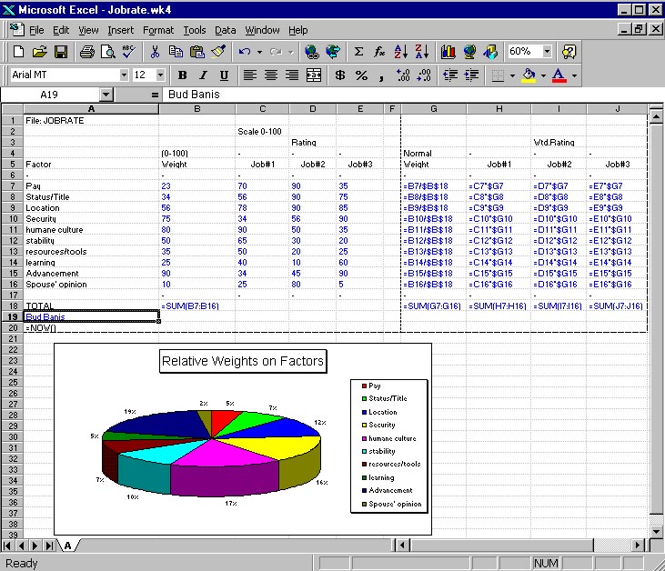
A) Put in weighted ratings for each job. Enter your weights in column B for each factor and the rating you would give each job on each factor in columns C, D, and E, respectively. Attach a printout showing which job rated highest for you. (15 points)

B) For each of the two rejected jobs: use the sheet to explore what changes you would have to get to make each of these your preferred option. For example, would higher pay or a contract (security) sway your decision? provide printouts for each of these scenarios commenting on the changes required to get you to change your mind in each case. (10 points for data, 5 points for discussion)

C) Attach a printout showing cell formulae rather than values by formatting all the cells to text. (15 points-depends on whether you did the formulas the hard way or the easy way)
D) Print a pie chart in the sheet to show the relative weights put on the different factors (5 points for some kind of graph)

Assembly of the sheet:
Row 18) has sums for each column. Note that the formula can be copied across once it's entered into cell B18. After doing this, you'll have to reformat the range G18..J18 to two decimal places.

G) Is a column of normalized weights derived from weights in column B. Each value in this column is equal to that factor's weight in column B divided by the sum of all factor weights in cell B18. The sum of column G (cell G18) should be 1.00. The whole column can be copied down from the right formula put in cell G7. To avoid a division by zero error, cell B18 must not be 0.

H through J) Are the weighted ratings for each alternative on each factor. These values result from multiplying each rating times the respective normalized weights. The right formula in cell H7 could be copied to the whole three column range.

There is a hard way and an easy way to put this sheet together. The hard way is to type each formula individually into each cell. The easy way is to design the formulae so that they are copiable to other cells, using a $ prefix to make references absolute where necessary, so that when you copy them they don't change. If it looks like you did it the easy way you'll get full credit.

The EXCEL COPY Command

When a formula is copied to another cell, references to other cells are changed to keep the same spatial relationship to the new cell.

In some cases, you want to keep the same absolute references. To keep a reference from changing when copied to a new cell, put a "$" in front of that part of the reference (row or column) that you want to keep absolute.

Here are some examples of results obtained from the COPY command with row or column references kept absolute. The original cell that was copied to the four-cell range is shown in yellow. 

• return to Bud's page